See here for the code.
During the summer semester 18, I had the opportunity to take part in the practical course ‘Large-scale Machine Learning’ offered by Prof. Guennemann at TUM. In my team, consisting of four people, we worked on mining public transport data in Munich provided by the company running the buses and trams (MVG).
Almost every household in Munich is located within 400 meters of an underground or tram station or a bus stop. The resulting network adds up to more than 587 km of routes for buses and trams only, which are served by 461 vehicles that stop approximately 345,000 times a day and log their position and status every few seconds.
The available data consists of GPS measurements, odometry readings plus door as well as stop events which were taken in the time period of January to May 2018.
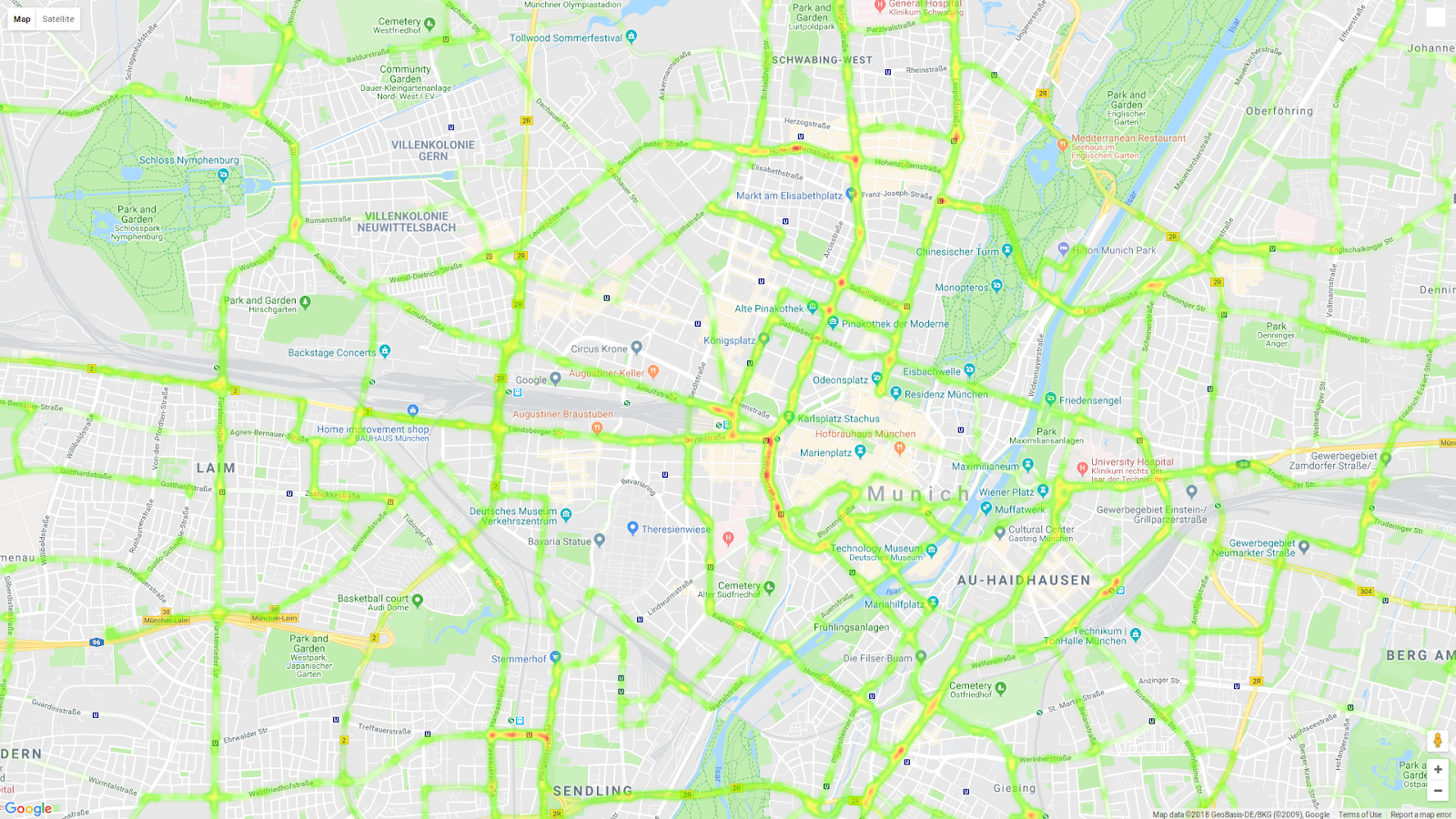
Raw GPS data heatmap plot.
Goal and Motivation
The goal of our project was to create an automatic network mapping pipeline. Up to now, a hand-crafted map is maintained by employees of the MVG. It shows the exact paths the vehicles take through the city which are frequently changing due to construction or replanning. A data-driven map has the advantage that it does not require constant maintenance and can be generated for example out of the data of a single week.
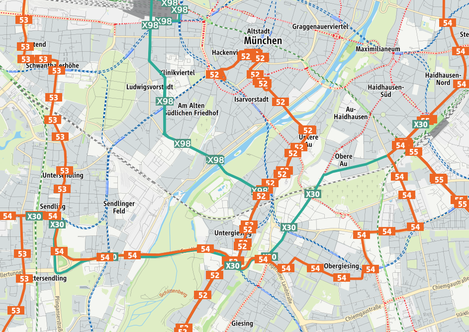
Hand-crafted map of public transport in Munich available [here](https://efa.mvv-muenchen.de/index.html#trip@enquiry).
Once such a map is available, many secondary tasks become feasible like detour detection or day time dependent mapping. Our requirements were:
- High accuracy of the map within two meters of real bus and driving lanes.
- Stops are spatially characterized by a 1D distribution around the mean.
- Automatic creation from the data with least human intervention as possible.
- Use shared information of different routes.
The spatial distribution of stops is especially important because many features of the buses like automatic stop announcements are based on relative distances between events. Those distances can be extracted out of our data-driven map which contains the spatial distribution of every stop.
Creating the Map
Our creating the map approach draws its main inspiration form the paper “A graph-based approach to vehicle trajectory analysis” published in the Journal of Location Based Services. We modified key elements to fit our specific task.
1. Applying a window averager to the raw data
A window average filter moves a position measurements to the mean of its neighbors within a certain radius. An important distinction we make is that we also match based on the driving direction which enables us to keep two close lanes in opposite directions separate. The result is a concentration of the positions at the local mean which corresponds to the driving lanes. As the GPS noise is unbiased this is a valid step which is validated by visual results.
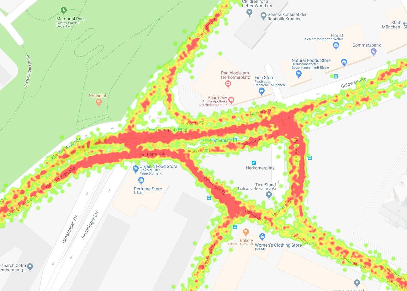
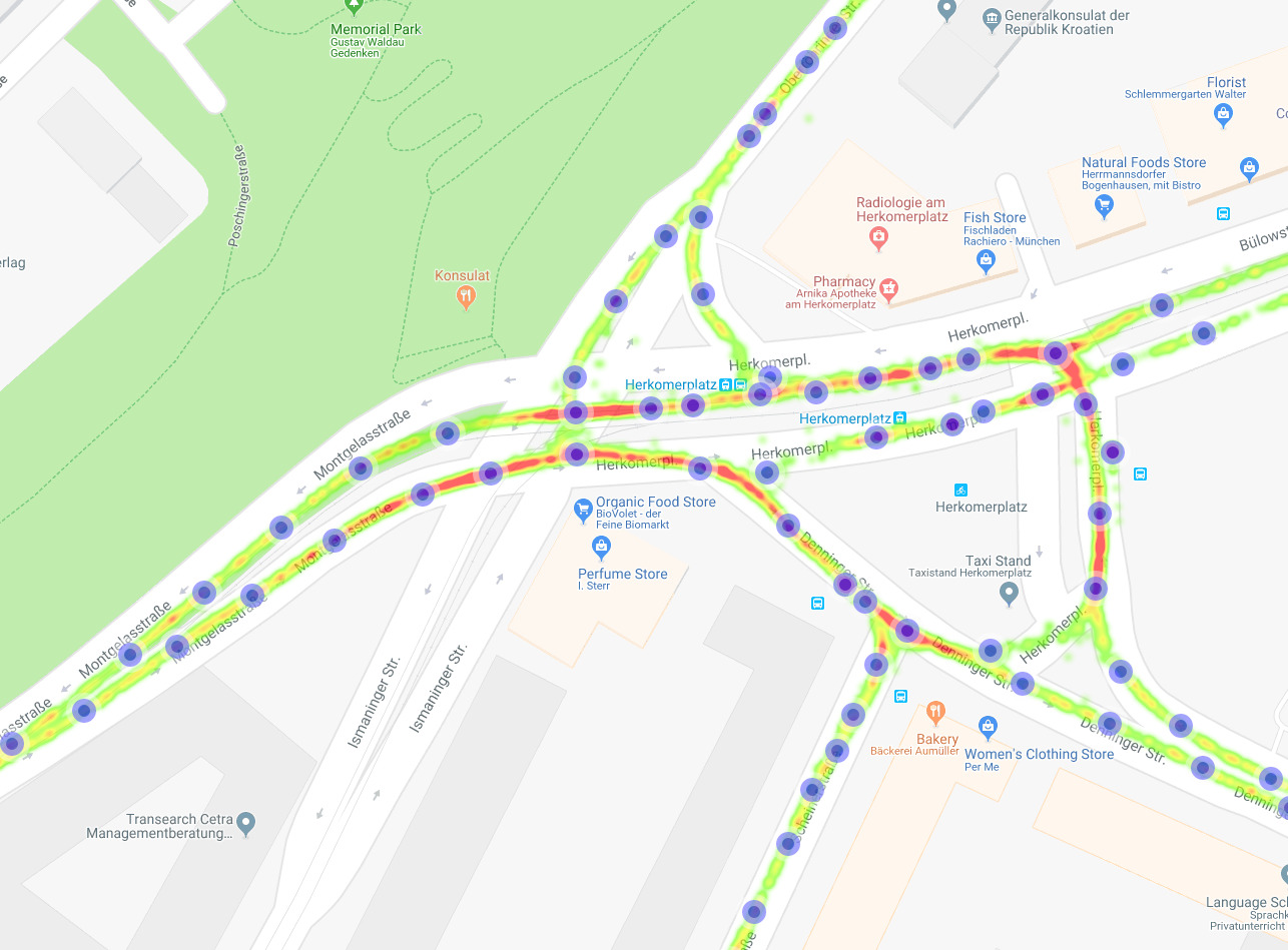
Raw GPS data at a crossing of more than two trams and buses
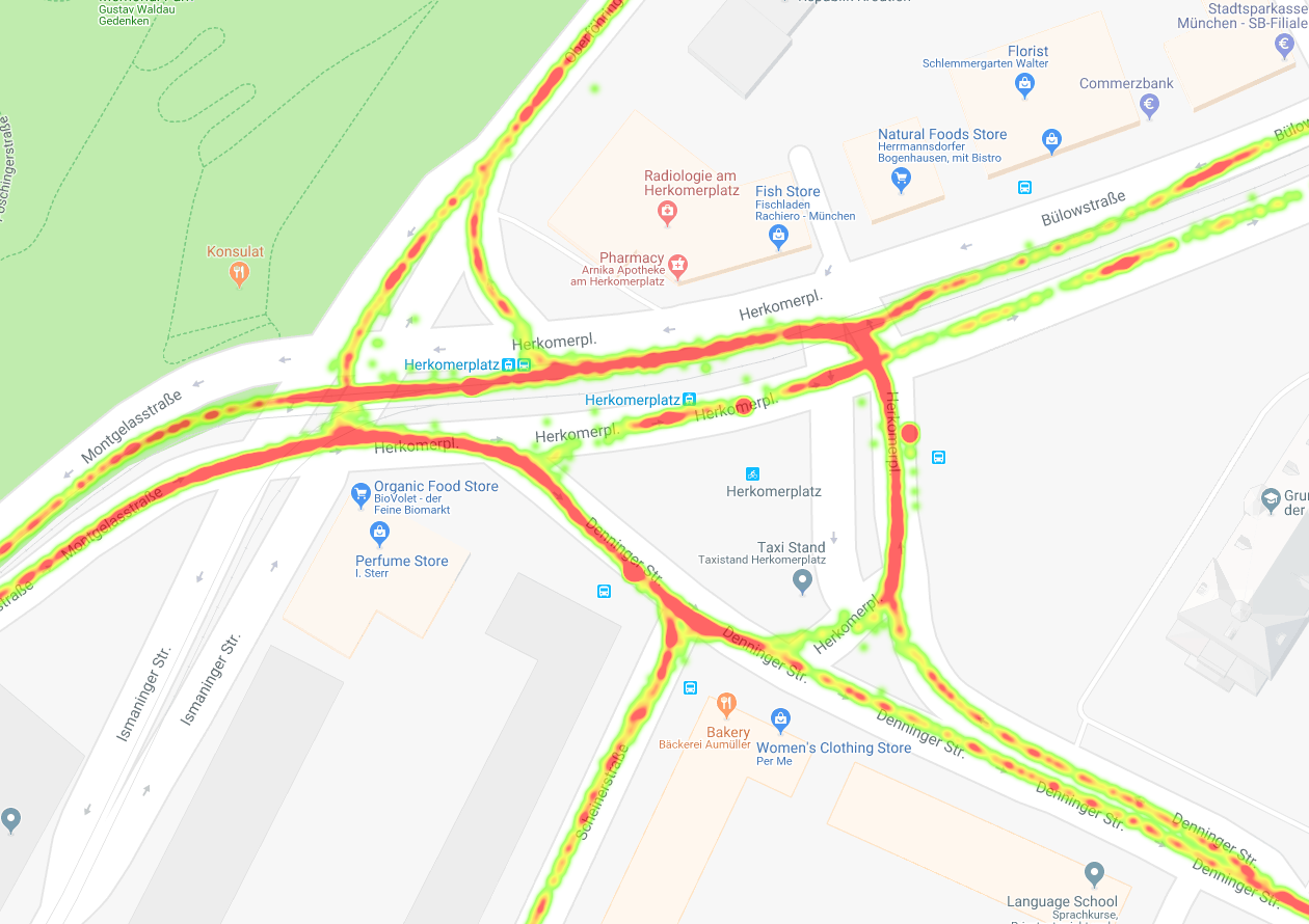
After applying a window average filter.
2. Finding representative centroids
The next step is to find representative measurements (centroids) which capture the overall trajectory of the route. We follow the six steps below:
- Start from any pose node s and let C=∅ be the set of representative centroids.
- Find all nodes within a certain threshold radius around s that are not represented yet by any centroid and have similar heading. Calculate the centroid position c_i as the mean of all these points.
- Find all nodes within a certain threshold radius and similar heading around c_i and a) assign them to c_i if they are not represented yet or b) calculate the distance to the old as well as new centroid and reassign it to the closer one.
- Choose next point s which is a neighbor of any point (Delaunay triangulation) within the current centroid c_i and is yet unrepresented. If no point fulfills the condition, pick a new unrepresented point randomly.
- Repeat steps (2) - (4) until all GPS points are represented.
- The centroids mean values are the new positions.
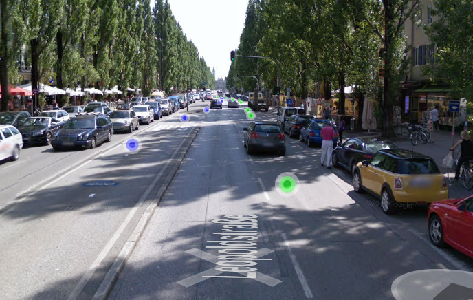
Representative centroids (blue dots) out of the filtered measurements.
3. Connecting the centroids
As we want to have a graph structure, it is necessary to connect the centroids. For this purpose we use the original sequential vehicle trajectories and connect all centroids which contain originally sequential measurements. This gives a graph which is very densely connected and which has to be “cleaned up” in the next step.
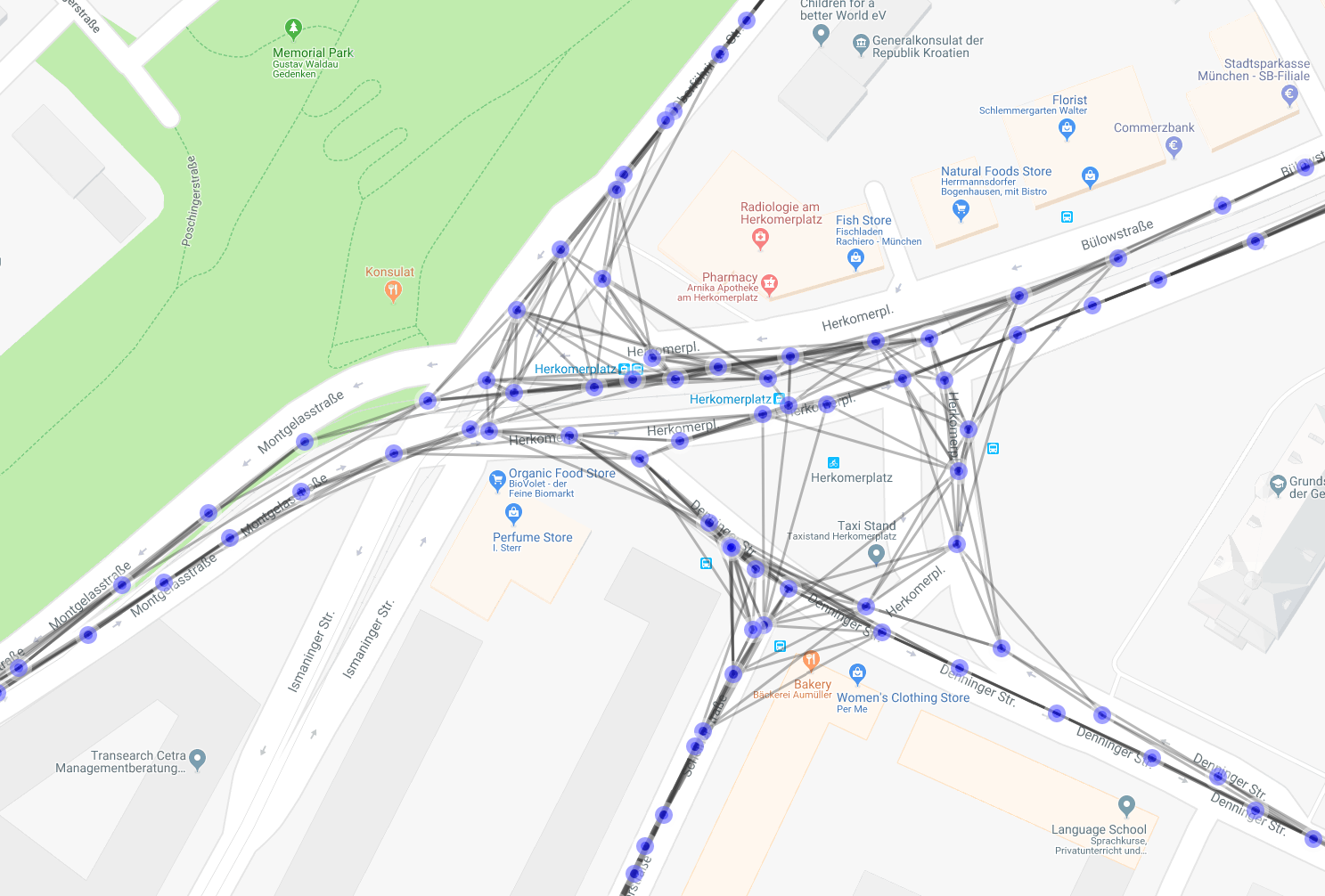
Connected centroids through sequential original measurements.
4. Sparsifying the edges
To connect the centroids in a reasonable way, we conduct a shortest path dijkstra search on the intermediate graph for each edge which has been added before. As the edge weight, a power of the euclidean distance is used with the exponent > 1. A value of two seems reasonable after some experimenting. The result is that the search prefers connections which use closer centroids instead of jumping directly over centroids.
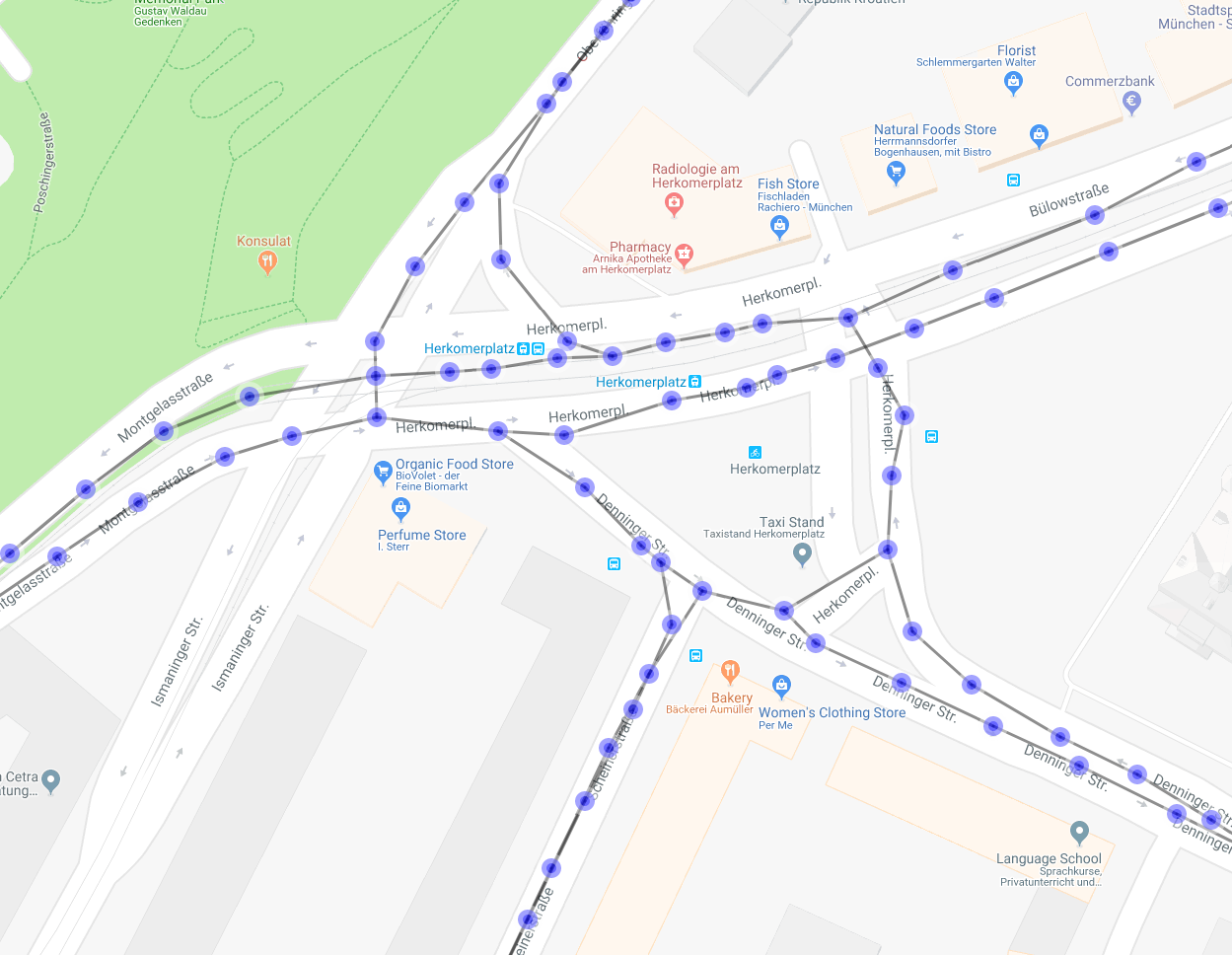
Edge sparsified graph / map
Centroid sparsification
One last step consists of dropping centroids on straight line segments as they do not provide additional spatial information. This is realized through the Ramer-Douglas-Peucker algorithm (RMP) which is already implemented through a python package and gives nice results.
Before sparsification
After sparsification
Map / Graph Evaluation
The huge amount of raw data measurements has to be compressed in a reasonable large map data structure. Our data-driven map achieves this goal through iterated sparsification steps which drop inexpressive data. The data reduction is shown below for an example map.
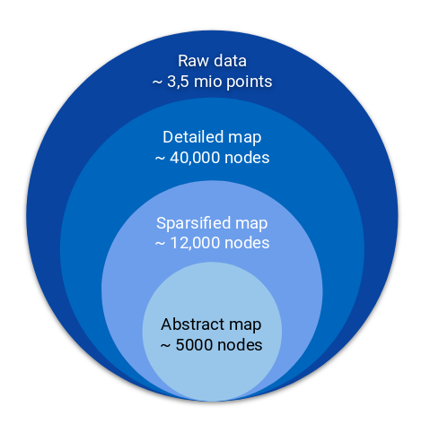
Data reduction in the map creation process.
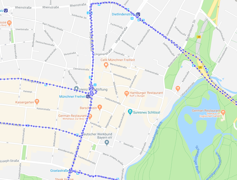
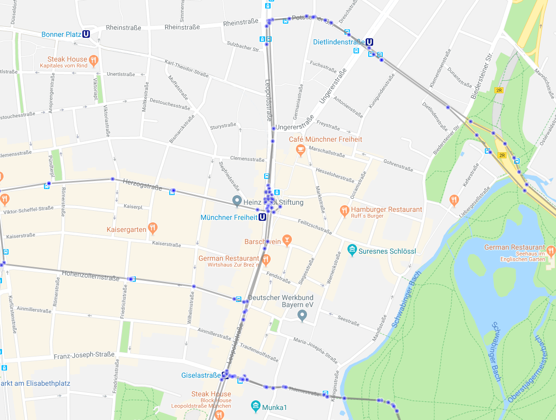
Overlaying the map onto satellite pictures shows very accurate mapping which clearly follows the designated bus lanes.
Below we can see that the hand-crafted map (green dots) is NOT located on the bus lane whereas our data-driven map nicely captures the in reality used driving lane.
Data-driven map (blue) better than hand-crafted map (green).
The stop information is contained in the map and can easily be visualized.
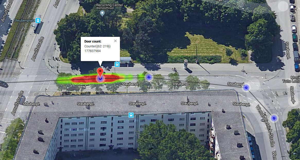
Stop distribution.
Conclusion
In this post, I described a complete data-driven network mapping approach for public transport based on our work in the course. You can find additional information in the code repository. Unfortunately, as the data is private and sensitive, I cannot provide a working example.