See github for code and my thesis as a pdf.
For my bachelor thesis, I had the opportunity to work for six months at the Namerikawa Laboratory at Keio University in Tokyo, Japan. The contact came through my professor Oliver Sawodny at the Institute for System Dynamics at the University of Stuttgart where I did my undergraduate studies. The lab focuses mainly on distributed control topics in the field of smart grids but also with agents such as drones
Problem Statement
Given is a moving formation which refers to a group of vehicles which have assigned relative positions to a shared reference coordinate system. When this reference coordinate system moves, the formation moves.
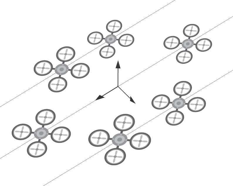
Movements of the reference coordinate frame result in different accelerations depending on the position of the individual vehicles in the formation. Below, the exemplary case of a rotation in 2D is shown where the orange diamonds indicate vehicle positions and the arrows direction as well as magnitude of the required acceleration.
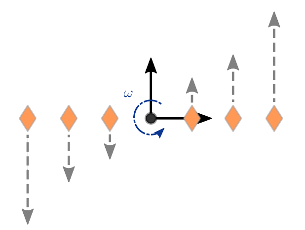
Real world vehicles have only limited acceleration capabilities. Consequently, the formation is corrupted when the reference frame performs fast rotational movements. The problem I tried to address in my thesis was how can we correct the reference frame movement in such a way that the acceleration limits of each vehicle in the formation are maintained. If this is not considered, problems like shown in the video below come up. The vehicles indicated by the colored diamonds should stay in a line formation which moves through space (orange bar). When the reference positions start to rotate the vehicles lack behind and consequently collapse to a single position because they already reached their upward maximal acceleration.
As the usage of swarms of vehicles becomes more likely in the future due to ongoing miniaturization and falling costs, the problem seems relevant for large scale formation movements.
Vehicle Modelling
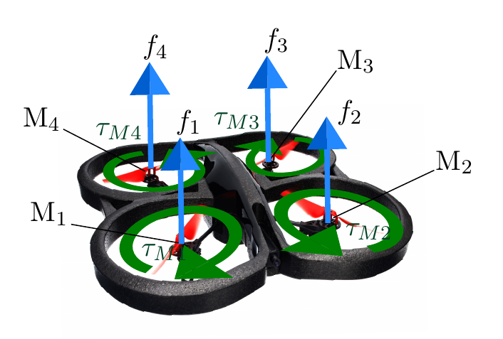
For my thesis, I chose quadrocopters / drones as the vehicles as they allow 3D movements in space and can be easily modeled. After simplifications, they can be modeled as two double integrator systems. They can be controlled using two nested PD controllers. For a detailed derivation refer to my thesis. As the main focus of the work was the distributed consensus reference control, the vehicle model is overly simplified. It only provides a basis to test the reference frame controller.
From the equations of motion of the system, acceleration limits depending on the current velocity of the vehicle can be calculated. Let
$$ a_\mathrm{quadpos} = \begin{bmatrix} \ddot{x}_\mathrm{max} & \ddot{y}_\mathrm{max} & \ddot{z}_\mathrm{max} \end{bmatrix}^T $$
be the positive acceleration limit and
$$ a_\mathrm{quadneg} = \begin{bmatrix} \ddot{x}_\mathrm{min} & \ddot{y}_\mathrm{min} & \ddot{z}_\mathrm{min} \end{bmatrix}^T $$
the negative acceleration limit expressed in Cartesian coordinates.
Reference Frame Controller
The reference frame state consisting of its position and orientation can be described in 3D by the state vector
$$ \boldsymbol{\xi}^r_\mathrm{contr} = \begin{bmatrix} x_r & y_r & z_r & \alpha_r & \beta_r & \gamma_r \end{bmatrix} ^T $$
where the first three entries are the position followed by Euler angles. \(\xi^r\) and its derivatives have to be controlled in such a way that all required acceleration are within the vehicle acceleration which can be concisely expressed as two inequalities
$$ a_\mathrm{quadneg} \leq a_\mathrm{max_2} \leq a_\mathrm{quadpos} $$
$$ a_\mathrm{quadneg} \leq a_\mathrm{max_1} \leq a_\mathrm{quadpos}. $$
To achieve this we define a controlled reference state
$$ \boldsymbol{\xi}^r_\mathrm{contr} = \begin{bmatrix} x_c & y_c & z_c & \alpha_c & \beta_c & \gamma_c \end{bmatrix} ^T. $$
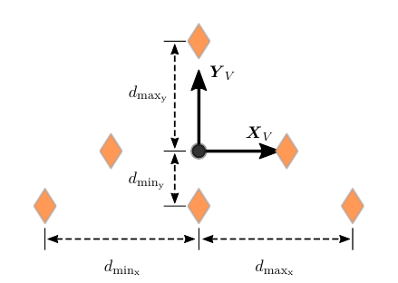
The maximum accelerations in a formation occur at the outermost vehicles in each coordinate direction as shown in the picture below. Therefore, this maximum distance information is provided to the reference controller through the state
$$ \boldsymbol{\zeta}i = \begin{bmatrix} d\mathrm{max} & d_\mathrm{min} \end{bmatrix} ^T $$
which is derived from the spatial desired formation.
The maximum occurring accelerations are calculated as
$$ a_\mathrm{max_1} = \ddot{r}_c + \dot{\omega} \times d_\mathrm{max} + \omega \times ( \omega \times d_\mathrm{max} ) $$
$$ a_\mathrm{max_2} = \ddot{r}_c + \dot{\omega} \times d_\mathrm{min} + \omega \times ( \omega \times d_\mathrm{min} ) $$
Now we have all the information available to finally build our complete reference controller. We want to minimize the deviation between $\xi^r_\mathrm{contr}$ and $\xi^r$ but still fulfill the inequalities. The controlled reference state dynamics are a double integrator. To control it we apply a simple PD control with an additional degree of freedom $c_a$. This input is used to add or subtract from the control output. The full dynamics of the reference controller are
$$ \ddot{\xi}^r_\mathrm{contr} = \ddot{\xi}^r + k^r_d \left(\dot{\xi}^r - \dot{\xi}^r_\mathrm{contr} \right) + k^r_p \left(\dot{\xi}^r - \dot{\xi}^r_\mathrm{contr} \right) + c_a $$
and a complete scheme is
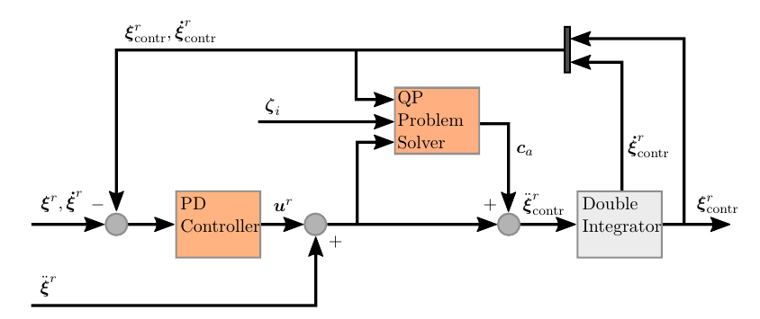
The final part is how to we calculate $c_a$? From the acceleration inequalities are linear inequalities. Furthermore we want to minimize $c_a$ in general, as we want to keep this artificial “disturbance” minimal. All of these points can be addressed by solving a simple QP problem which is convex and has a unique global solution. As the dimensionality is small with $c_a \in \mathcal{R}^6$, solving the optimization in each time step is feasible. The QP problem solver is only active if the acceleration is about to exceed its limits, otherwise $c_a = 0$.
Results
The 2D formation flight with rotation shown at the beginning can now be simulated with active reference control. The video below shows that when the reference frame start to rotate it clearly slow down which allows the outermost vehicles to stay within the physical limits.
We can extend the setup to a 3D case where the pink cube now represents the reference frame position and orientation. Without the active reference controller we get a similar picture as in the 2D case where the formation collapses
With active reference controller, the reference trajectory is modified in such a way that we stay within the limits of the vehicles but still try to follow the given path best as possible
Conclusion
I hope you enjoyed this little read-up on my thesis. As stated in the beginning, you can find an in-depth derivation of most of the concepts in the thesis and the code is provided github.